Geir K. Pedersen's research while affiliated with University of Oslo and other places

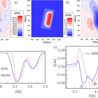
Free wave generation due to a ship or storm moving past a shallow, great depth change of the water, is measured on the shore (coast), modeled and compared. The free waves are generated at the depth change where the forced wave and velocity field attached to the moving pressure system adjust to the new depth. The wavenumber is a factor 1/12 smaller in the meteotsunami case compared to the ship case. The subcritical depth Froude numbers are similar in the two cases. The meteotsunami that occurred on the Norwegian Coast on 29–30 June 2019 was driven by a supercell thunderstorm moving at speed 110 km/hr. A localized, strong high pressure feature of width of 60 km and crest of 120 km obtained from weather forecast was used as input for a set of simulations of the water‐level response including realistic bathymetry. At the transition between the North Sea and the Norwegian Trench, the storm generated a free depression wave. This arrived at the coast 24 min ahead of the depression attached to the storm. The calculation fits to a period of 23 min, of a series several oscillations of height of 0.3–0.4 m, as measured by the water‐level gauge. An impulsive start‐up generates an additional forerunning elevation wave. Short waves of period of 1/3 of the main ship‐driven waves may originate from the steep gradients of the bow and stern. Similarly, short waves of period 6–7.5 min (0.002–0.003 Hz) are observed in the measured water‐level on the coast.

The 2018 Anak Krakatoa volcano flank collapse generated a tsunami that impacted the Sunda Strait coastlines. In the absence of a tsunami early warning system, it caused several hundred fatalities. There are ongoing discussions to understand how the failure mechanism of this event affected landslide dynamics and tsunami generation. In this paper, the sensitivity to different failure scenarios on the tsunami generation is investigated through numerical modelling. To this end, the rate of mass release, the landslide volume, the material yield strength, and orientation of the landslide failure plane are varied to shed light on the failure mechanism, landslide evolution, and tsunami generation. We model the landslide dynamics using the depth-averaged viscoplastic flow model BingClaw, coupled with depth-averaged long wave and shallow water type models to simulated tsunami propagation. We are able to match fairly well the observed tsunami surface elevation amplitudes and inundation heights in selected area with the numerical simulations. However, as observed by other authors, discrepancies in simulated and observed arrival times for some of the offshore gauges are found, which raises questions related to the accuracy of the available bathymetry. For this purpose, further sensitivity studies changing the bathymetric depth near the source area are carried out. With this alteration we are also able to match better the arrival times of the waves.

The 2018 Anak Krakatoa volcano flank collapse and tsunami caused several hundred fatalities. There was no early warning system in place for the landslide triggered tsunami, and there is a lack in understanding on how the failure mechanism affected landslide dynamics and tsunami generation, which we focus on in this study. While researchers previously have modelled the collapse as an instantaneous release, we here illuminate how different landslide failure scenarios, including a gradually released flank failure, influence the tsunami generation. We simulate the material movement by using a viscoplastic flow model with Herschel-Bulkley rheology and we employ a depth-averaged model to both the landslide and the tsunami propagation. A sensitivity study to the gradual mass release, total release volume, the material yield strength, the remoulding coefficient, and landslide directivity is used to shed light on the tsunami generation. Our analysis indicates that an instantaneous mass release in 125 degree SW direction fits the observed waveforms at coastal gauge stations best. In our simulations, we observe, as many other authors, discrepancies between simulated and observed arrival times and wave periods offshore Sumatra. Hence, we have also investigated sensitivity to the bathymetric depth by varying the water depth in areas near the source. Finally, we simulate the tsunami inundation at two coastal sites in southwestern Java using open-source topographic data. Given the limitations in the topographic data, a reasonably good agreement between the simulations and observations are obtained.

Sediment slumps are known to have generated important tsunamis such as the 1998 Papua New Guinea (PNG) and the 1929 Grand Banks events. Tsunami modellers commonly use solid blocks with short run-out distances to simulate these slumps. While such methods have the obvious advantage of being simple to use, they offer little or no insight into physical processes that drive the events. The importance of rotational slump motion to tsunamigenic potential is demonstrated in this study by employing a viscoplastic landslide model with Herschel–Bulkley rheology. A large number of simulations for different material properties and landslide configurations are carried out to link the slump’s deformation, rheology, its translational and rotational kinematics, to its tsunami genesis. The yield strength of the slump is shown to be the primary material property that determines the tsunami genesis. This viscoplastic model is further employed to simulate the 1929 Grand Banks tsunami using updated geological source information. The results of this case study suggest that the viscoplastic model can be used to simulate complex slump-induced tsunami. The simulations of the 1929 Grand Banks event also indicate that a pure slump mechanism is more tsunamigenic than a corresponding translational landslide mechanism.

Tsunamis are natural hazards that can be caused by submarine landslides. Landslides with short run-out and duration are called slumps, and their tsunami generation have commonly been modelled simplistically by using blocks. The block approach was used for modelling tsunamis of important historical events such as the 1998 Papua New Guinea (PNG) and the 1929 Grand Banks. While such a method has the advantage of being simple to use, it offers no or little insight into physical processes like ductile deformation of the sediments during the slump motion. Here, we use a viscoplastic landslide model with Herschel-Bulkley rheology to model the deformable sediments on a simplified geometry. The sediment's yield strength is an important factor for the tsunami-genesis, and the resulting translational kinematics relate to the tsunami height as studies for long run-out landslides have already shown. In this study, we also show the importance of the rotational slump motion related to the tsunami-genesis, for the first time, by using a deformable slump. In addition to the idealized study, we use the same viscoplastic model to simulate the 1929 Grand Banks event under consideration of the updated slump source representation. The size of the tsunami simulated for the Grand Banks event modelling confirms that our viscoplastic model can be used for complex slump induced tsunamis. On the other hand, more work is needed to understand the exact generation mechanism.

In the present study, we analyse the influence of submarine slump source dynamics on tsunami generation. Slump induced tsunamis have traditionally been treated using block sources with prescribed velocities as tsunami sources, such as for describing the tsunami generation due to important historical events like the 1998 Papua New Guinea and the 1929 Grand Banks events. However, our intention is to model the slump motion as a viscoplastic flow where the material behaviour determines the landslide dynamics directly. To this end, we use a new landslide model labelled BingClaw that incorporates a Herschel-Bulkley rheology, formulated numerically in a depth-averaged Riemann formulation. For the wave propagation we use the Boussinesq equations including linear and dispersive effects, conveying the landslide tsunami generation using full potential flux sources. We alter mechanical soil parameters such as yield strength, dynamic viscosity, flow exponent, as well as sea bed inclination below the sliding mass, and show relations between these parameters, angular momentum and bed parallel velocity of the sliding mass, and frontal wave height. We illustrate that weaker sliding materials that have lower viscosity, lower yield strength, higher flow exponent, and higher sea bed inclination, generate higher frontal wave heights. Finally, we show that the wave generation correlates with kinematic properties such as the landslide angular momentum and spin, which indicate how the rotational motion of the slump is important for the wave generation.

We reformulate the depth-averaged non-hydrostatic extension for shallow water equations to show equivalence with well-known Boussinesq-type equations. For this purpose, we introduce two scalars representing the vertical profile of the non-hydrostatic pressure. A specific quadratic vertical profile yields equivalence to the Serre equations, for which only one scalar in the traditional equation system needs to be modified. Equivalence can also be demonstrated with other Boussinesq-type equations from the literature when considering variable depth, but then the non-hydrostatic extension involves mixed space-time derivatives. In case of constant bathymetries, the non-hydrostatic extension is another way to circumvent mixed space-time derivatives arising in Boussinesq-type equations. On the other hand, we show that there is no equivalence when using the traditionally assumed linear vertical pressure profile. Linear dispersion and asymptotic analysis as well as numerical test cases show the advantages of the quadratic compared to the linear vertical non-hydrostatic pressure profile in the depth-averaged non-hydrostatic extension for shallow water equations.

The nonlinear shallow water model is widely used in the study of tsunami propagation, but an increasing number of studies are dedicated to the dispersion dynamics of tsunamis. If the wave dispersion becomes important, Boussinesq-type models are often used. In this work, a general purpose Boussinesq solver, BoussClaw, is introduced for modeling non-linear dispersive tsunami propagation, taking into account inundation. The BoussClaw model is an extension of the GeoClaw tsunami model. It employs a hybrid of finite volume and finite difference methods to solve Boussinesq equations from the literature, which are based on the depth-averaged velocity and include enhanced dispersion properties. On the other hand, in the selected formulation only some non-linearity is retained in the dispersion term. In order to validate BoussClaw, numerical results are compared to analytic solutions, solutions obtained by pre-existing models, and laboratory experiments. Even though the equations of BoussClaw are not fully nonlinear they perform far better than standard Boussinesq equations with only linear dispersion terms. Furthermore, the wave steepening and breaking are carefully scrutinized, and we demonstrate that the point of wave breaking may be wrongly identified in many of the commonly used Boussinesq models.

This study presents an experimental investigation of plunging breakers on a sloping beach with an inclination of 5.1°. The incident waves are solitary waves with various amplitudes from non-breaking waves to plunging breakers, and the area investigated is the swash zone. PIV (Particle Image Velocimetry) is performed on images captured at four different field of views (FOV). Shoreline position and maximum runup are measured, and are repeatable in both time and height, although cross-sectional variations of the shoreline shape are observed at maximum runup. For non-breaking waves the runup and fluid flow is computed by a boundary integral technique combined with a boundary layer model. Then, there is excellent agreement between the experimental and the computed velocity profiles at the lower region of the beach, while the boundary integral technique overpredicts the maximum runup height severely. For breaking waves the experiments indicate that the motion becomes more irregular as we move further up the beach. In addition, there are more irregularities present for waves with larger amplitude. Length and velocity of air bubbles entrapped by the plunging breakers are extracted from an image series captured with a large FOV. The images showed that a large air bubble remains intact for a time period during runup for the breaking waves.

In the present treatise, a stability analysis based on energy bounds and nonmodal theory is performed. The instability mechanism of this flow consists of a competition between streamwise streaks and two-dimensional perturbations. For lower Reynolds numbers and early times, streamwise streaks display larger amplification due to their quadratic dependence on the Reynolds number, whereas two-dimensional perturbation become dominant for larger Reynolds numbers and later times in the deceleration region of this flow, as the maximum amplification of two-dimensional perturbations grows exponentially with the Reynolds number. By means of the present findings, the results by direct numerical simulation in (Vittori & Blondeaux 2008; Ozdemir et al. 2013) and experiments in (Sumer et al. 2010) can be explained and interpreted. In addition, three critical Reynolds numbers can be defined for which the stability properties of the flow change. In particular, it is shown that this boundary layer changes from an absolutely stable to a convectively unstable flow at a Reynolds number of 18.